Cancer Cell Dynamics

We have previously introduced a cancer cell propagation model in earlier discussions which others have also considered. However our model is for a single cell type which grows diffuses and flows. The rates of each are dependent on where the cell is.

In this brief note we add other elements, namely the probability that a cell can mutate and that as it mutates the factors related to the propagation model may also change. We calculate a similar diffusion equation now for the average number of malignant cells by region and by type. That is we demonstrate in the following graphic summary:

1. The standard diffusion-flow-proliferation model applies on a per-region and per cell type basis. This means that the constants we have developed previously will depend on the specific cell type as well, namely how many mutations have occurred.

2. That we know there are multiple mutations in cancer cells. Some may have a few and are indolent and others may have many and be aggressive. We develop a Markov model for such cell progression.

3. We combine the three element spatio-temporal model with the Markov cell mutation model and this allows us to determine the average number of cells of a specific type in any part of the body at any point in time.

4. We then discuss how one may use this model for prognostic and therapeutic purposes.

The main observation in this brief section is that the average number of malignant cells of a specific mutation state can be determined by the following:

 

 In this equation the n is an NX1 vector of average numbers in spatio-temporal dependent values of each of N possible mutations and the L value is the spatio-temporal dependent operator matrix and Λ is a matrix describing the Markov transition probabilities between mutations.

It should be clear that we can measure all of the constants involved and thus determine the result. As a counter-distinction we can measure the n values and mutation states and determine the constants.

The expanded model considers the issue diagrammed below:

The next issue is the ability to determine what the factors are in the specific model, namely the values of the constants, and secondly the validation of the model itself.

Thus there are two dimensions of issues here:

1. Model Identification and Validation: In previous work we referred to this as the Observability problem. Namely if we have a model and we can identify the required parameters, then can this model be used to determine the end state which will be attained. This is the prognostic problem.

2. Model Utilization: As with the previous cases, if we have this model, and we have identified the constants, can we determine actions which may be taken to control the end state of the system? This is the Controllability problem. It states that perhaps having such a model we can determine methods and means to drive the system, in this case the average number of malignant cells of genotype say G, to a new end state, one where we have reduced the number of bad cells to a de minimis level. This is the therapeutic problem.

There also is a third element:

3. Identification: In both of the two previous issues we assumed that there existed a method by which we could determine the constants of diffusion et al and furthermore that we could ascertain the list of possible mutations, and also their Markov transition probabilities. This may be accomplished in two ways. First, we can accomplish this by in vitro studies. Second, we can achieve this by using the model itself in a classic system identification model with in vivo analyses.

Thus the analysis contained herein is an initiation of what appears to be an innovative way to look at cancer. There have been many studies in more specific and segmented areas but there has not to my knowledge been a study that has examined cancer in such a broad and overarching manner. In essence we have included all of the variables that one may ask for.

To better understand we depict the progression of prostate cancer below.

Step 1: Benign State, here we have five segments; prostate, two tissue-blood barriers, blood, and bone.

 

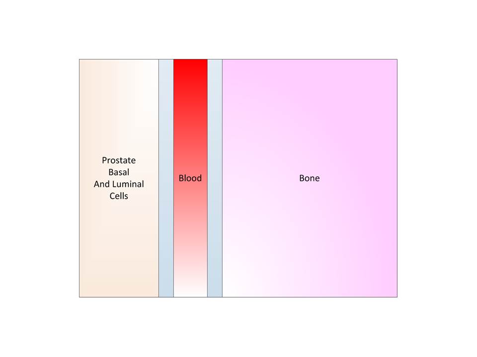
Step 2: We have the beginning of a cancer due to some mutation of the basal or luminal cells. The cancer proliferates and diffuses. It is still localized here.

 Step 3: Diffusions sends cancer cells to the blood barrier.

 Step 4: The blood barrier is crossed, and we assume by diffusion. Across this barrier there is no proliferation or flow, just diffusion.

 Step 5: The blood barrier is crossed and the cell is now in the blood stream. Here we have flow but no diffusion and no proliferation.

  Step 6: The blood barrier is crossed again as discussed above.

  Step 7: Metastasis is complete by having the new malignant cells in the bone and proliferation and diffusion predominate.

The above steps are common is almost all cancers. The assumptions here are:

1. The same malignant cell moves across the body.

2. Each separate area, in this case five, has constant diffusion, flow and proliferation constants.

3. That we can then measure the number of cells from this deterministic model.

In the case where they are uniform constants we can solve the equation. In the case where they are uniform constants across uniform spatial domains then we can also solve the equations evoking boundary conditions.

We now want to expand this model to include multiple malignant cell types. Also we want to include their stochastic dynamics as well.

Consider a cell with five possible mutations. We show the genes below. The call may begin with one mutation and then move to a second and so forth. Each path is assumed to be possible and the results of each path are different.

Now we can consider a model for the above simple example. We have 5 possible mutations and they may occur in any order. We assume they occur one at a time. We can identify any number of cells as n(x,t), as the number of cells after one mutation at location x and at time t, of mutation k.

Now we have the following observations:

1. At mutation 1 we have 5 possible cell mutants. Furthermore each may be considered a cancer cell and the growth, diffusion and flow are as described above. Some of the mutations may be indolent and some aggressive.

2. At mutation 2 we have 5*4 possible cells. The question is that some are say PTEN then cMyc or cMyc then PTEN. Are they the same, and this means the difference between perturbation and combination? Are they distinct by have been ordered differently or are they the same? If it is a combination we have 10 instead of 20 different mutations.

3. At mutation 3 we have 5*4*3 and at 4 we have 5*4*3*2 or 120 permutations.

4. At any location we may have any one or a combination of these mutation types. There are two factors driving their number:

a. A single type will have growth, dispersion and movement dynamics with the above mentioned model but each mutation will respond differently since their coefficients will be different. Some may grow faster and some may diffuse faster. There is no a priori ranking of the coefficients.

b. The surrounding mutant types will also tend to mitigate growth.

For example consider the following three gene mutation case:

 We can thus make several important observations regarding this model.

1. Prognostic and Therapeutic: We can determine the transitions and the factors related to diffusion, flow and growth. Thus we can use the result as a powerful one for prognostic and therapeutic results. As we had indicated earlier, the Observability and Controllability issues are essentially Prognostic and Therapeutic respectively.

2. Variances: The results are for the average. We can determine the results for the variances as well. We have examined the variances on the averages and they are somewhat complex and we do not believe that they lend significant additional information at this time.

3. Solutions: The solutions to these equations are readily obtained using standard techniques. They can, in addition, be determined in closed form results.